Quickstart

Basic inference

The easiest way to get started is by using the BaseInference class which infers the DFE from a single pair of frequency spectra, one neutral and one selected. In this example we create Spectrum objects holding the SFS counts and pass them to BaseInference. Note that we are required to specify the number of monomorphic sites (the last and first entries of the specified counts which correspond to the number of mono-allelic sites where the ancestral and derived allele is fixed, respectively).

library(fastdfe)

# load the fastdfe package
fastdfe <- load_fastdfe()

# import classes
BaseInference <- fastdfe$BaseInference
Spectrum <- fastdfe$Spectrum

# configure inference
inf <- BaseInference(
  sfs_neut = Spectrum(c(177130, 997, 441, 228, 156, 117, 114, 83, 105, 109, 652)),
  sfs_sel = Spectrum(c(797939, 1329, 499, 265, 162, 104, 117, 90, 94, 119, 794))
)

# run inference
sfs_models <- BaseInference$run(inf)

fastDFE uses maximum likelihood estimation (MLE) to find the DFE. By default, 10 local optimization runs are carried out to make sure a reasonably good global optimum has been bound. The DFE furthermore needs to parametrized where GammaExpParametrization is used by default.

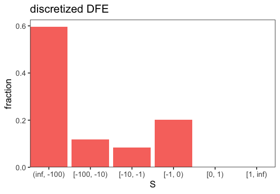
We can now plot the inferred DFE in discretized form (cf. plot_discretized()).

p <- BaseInference$plot_discretized(inf)

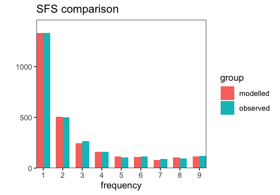
We can also plot a comparison of the (selected) modelled and observed SFS (cf. plot_sfs_comparison()).

p <- BaseInference$plot_sfs_comparison(inf)

Bootstrapping

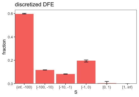
We can perform parametric bootstrapping (cf. bootstrap())

bs <- inf$bootstrap()

# redo the plotting
p <- BaseInference$plot_discretized(inf)

Serialization

# save the inference object to the file
# we can unserialized the inference by using BaseInference.from_file
inf$to_file("out/serialized.json")

# alternatively we can also save a summary to file
inf$get_summary()$to_file("out/summary.json")