DFE inference

Base inference

In order to infer the DFE of a single pair, one neutral and one selected, we can use BaseInference. In this example we create Spectrum objects holding the SFS counts and pass them to BaseInference. Note that we are required to specify the number of monomorphic sites (the last and first entries of the specified counts).

library(fastdfe)

# load the fastdfe package
fastdfe <- load_fastdfe()

# import classes
BaseInference <- fastdfe$BaseInference
Spectrum <- fastdfe$Spectrum

sfs_neut <- Spectrum(c(177130, 997, 441, 228, 156, 117, 114, 83, 105, 109, 652))
sfs_sel <- Spectrum(c(797939, 1329, 499, 265, 162, 104, 117, 90, 94, 119, 794))

# create inference object
inf <- BaseInference(
    sfs_neut = sfs_neut,
    sfs_sel = sfs_sel,
    n_runs = 10
)

# run inference
sfs_modelled <- BaseInference$run(inf)

fastDFE uses maximum likelihood estimation (MLE) to find the DFE. By default, 10 local optimization runs are carried out to make sure a reasonably good global optimum has been bound (see BaseInference for all configuration options). The DFE furthermore needs to parametrized where GammaExpParametrization is used by default.

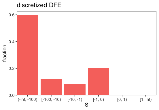
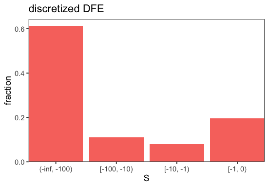
We can now plot the inferred DFE in discretized form (cf. plot_discretized()).

p <- BaseInference$plot_discretized(inf)

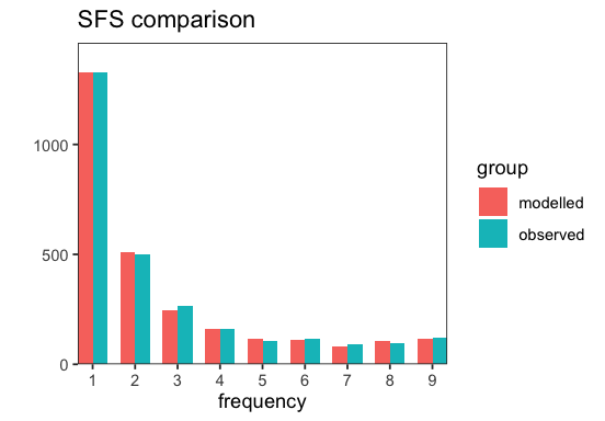
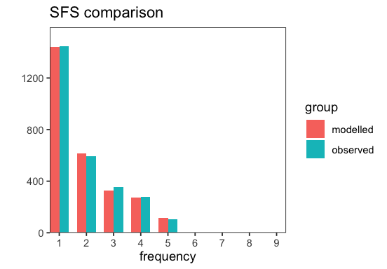
We can also plot a comparison of the (selected) modelled and observed SFS (cf. plot_sfs_comparison()).

p <- BaseInference$plot_sfs_comparison(inf);

Bootstrapping

We can perform parametric bootstrapping (cf. bootstrap()) to estimate the uncertainty of the inferred DFE. This is done by sampling new SFSs from the inferred DFE and re-running the inference.

# run bootstrapping
bootstraps <- BaseInference$bootstrap(inf, n_samples = 100)

# redo the plotting
p <- BaseInference$plot_discretized(inf)

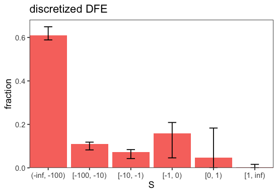
The bars indicate 95% confidence intervals. We can adjust the confidence level among other things (cf. plot_discretized()).

Fixing parameters

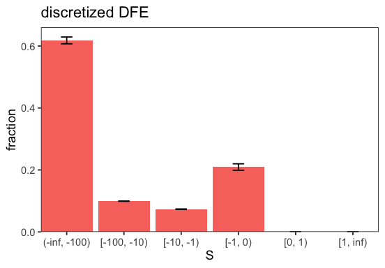
We can hold parameters fixed during the maximum likelihood optimization. This is useful, for example, if only using a subset of the parameters has a reasonable interpretation. In this example, we fix ancestral-allele mis-identification rate eps to 0. We also force the DFE to be purely deleterious, by fixing S_b to some arbitrary value and setting p_b to 0 (cf. GammaExpParametrization).

# create inference object
inf <- BaseInference(
    sfs_neut = sfs_neut,
    sfs_sel = sfs_sel,
    # Fix parameters, note that we need specify type 'all'
    # if only one type is used. Later we will work with
    # more than one type.
    fixed_params = list(all=list(eps=0, S_b=1, p_b=0)),
    do_bootstrap = TRUE
)

# run inference
sfs_modelled <- BaseInference$run(inf)

p <- BaseInference$plot_discretized(inf);

Nested model comparison

We can automatically check for the significance of include ancestral-allele mis-identification and beneficial fitness affects using likelihood ratio test (LRTs). This is done with plot_nested_models(). The LRTs are performed by comparing the likelihood of the inferred DFE to the likelihood of a nested model where some parameters are held fixed.

p <- BaseInference$plot_nested_models(inf)

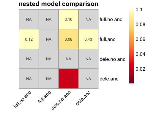
Including ancestral allele mis-identification appears to improve the fit significantly when modelling the deleterious DFE.

Visualize likelihoods

We can visualize the likelihoods of the differently-initialized optimization runs. This can give us some information on how good an optimum could be found.

p <- BaseInference$plot_likelihoods(inf, scale = 'lin')

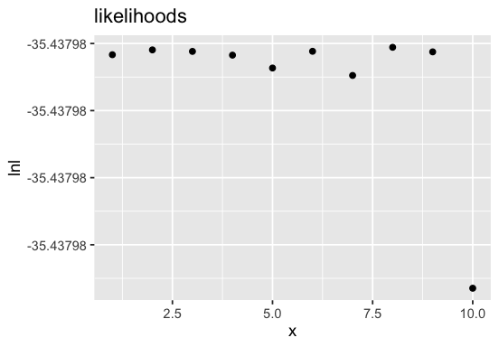
There might be some room for improvement as the likelihoods do show some variation. We could consider increasing the n_runs argument.

Serialization

# save the inference object to a file
# unserialize with BaseInference$from_file
BaseInference$to_file(inf, "serialized.json")

# we can also save a short summary to fa ile
BaseInference$get_summary(inf)$to_file("summary.json")

Folded inference

To infer the DFE from a folded SFS, simply pass folded spectra to BaseInference. Folded inference is performed whenever the spectra appear to be folded, i.e., when all entries where the derived allele is the major allele are zero. In this example, we only infer the deleterious DFE as folded spectra contain no information on beneficial mutations.

# create inference object
inf <- BaseInference(
    sfs_neut = Spectrum$fold(sfs_neut),
    sfs_sel = Spectrum$fold(sfs_sel),
    fixed_params = list(all = list(eps = 0, S_b = 1, p_b = 0))
)

# run inference
sfs_modelled <- BaseInference$run(inf)

p <- BaseInference$plot_discretized(inf, intervals = c(-Inf, -100, -10, -1, 0))

p <- BaseInference$plot_sfs_comparison(inf)

Joint inference

fastDFE supports joint inference of several SFS types, where any parameters can be shared between types. In this example, we create a JointInference object with two types, where we share eps, the rate of ancestral misidentification and S_d, the mean selection coefficient for deleterious mutations (cf. GammaExpParametrization). For more complex stratifications, see the Parser) module.

joint_inference <- fastdfe$JointInference
spectra <- fastdfe$Spectra
shared_params <- fastdfe$SharedParams

# neutral SFS for two types
sfs_neut <- spectra(list(
    pendula = c(177130, 997, 441, 228, 156, 117, 114, 83, 105, 109, 652),
    pubescens = c(172528, 3612, 1359, 790, 584, 427, 325, 234, 166, 76, 31)
))

# selected SFS for two types
sfs_sel <- spectra(list(
    pendula = c(797939, 1329, 499, 265, 162, 104, 117, 90, 94, 119, 794),
    pubescens = c(791106, 5326, 1741, 1005, 756, 546, 416, 294, 177, 104, 41)
))

# create inference object
inf <- joint_inference(
    sfs_neut = sfs_neut,
    sfs_sel = sfs_sel,
    shared_params = list(shared_params(types = c("pendula", "pubescens"), params = c("eps", "S_d"))),
    do_bootstrap = TRUE
)

# run inference
sfs_modelled <- joint_inference$run(inf)

JointInference both runs the joint inference and marginal inference where each type is inferred separately. To see this better we can plot the inferred parameters for the different inference types.

p <- joint_inference$plot_inferred_parameters(inf)

Scale for y is already present.
Adding another scale for y, which will replace the existing scale.

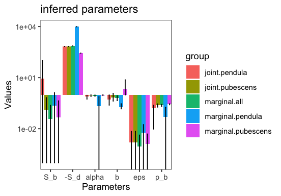
marginal.pendula and marginal.pubescens are the marginal inferences for the respective type. marginal.all is the marginal inference obtaining by adding up the spectra of all types. joint.pendula and join.pubescens are the joint inferences for the respective type. We can see that eps and S_d are indeed shared between the two. The parameter alpha in the plot denotes the proportion of beneficial non-synonymous substitutions. Each marginal inference is a BaseInference object itself and can be accessed via inf.marginal_inferences[type].

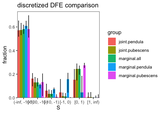
We can now also investigate to what extent the inferred DFEs differ:

p <- joint_inference$plot_discretized(inf)

Model comparison

We can obtain information about the goodness of fit achieved by sharing the parameter by performing a likelihood ratio test (cf. perform_lrt_shared()). This compares the likelihood of the joint inference with the product of the marginal likelihoods.

joint_inference$perform_lrt_shared(inf)

0.647012595655615

The test is not significant, indicating that the simpler model of sharing the parameters explains the data sufficiently well. Indeed, we do not observe a lot of differences between the inferred parameters of joint and the marginal inferences.

Covariates

JointInference also supports the inclusion of covariates associates with the different SFS types. This provides more powerful model testing and reduces the number of parameters that need to be estimated for the joint inference. For a more interesting example we stratify the SFS of B. pendula by the sites’ reference base as is described in more detail in the parser module.

parser <- fastdfe$Parser
spectra <- fastdfe$Spectra

# instantiate parser
p <- parser(
    n = 10,
    vcf = paste0(
        "https://github.com/Sendrowski/fastDFE/",
        "blob/dev/resources/genome/betula/",
        "all.polarized.deg.subset.200000.vcf.gz?raw=true"
    ),
    stratifications = list(fastdfe$DegeneracyStratification(), fastdfe$AncestralBaseStratification())
)

# parse SFS
s <- parser$parse(p)

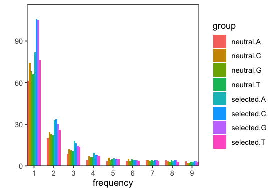
# visualize spectra
p <- spectra$plot(s)

We now create the inference object from the spectra. In this contrived example we make up some covariates that covary with S_d, the mean strength of negative selection. Covariates introduce a linear relationship by default but this can be modified by specifying a custom callback function (see Covariate).

covariate <- fastdfe$Covariate

# create inference object
inf <- joint_inference(
    sfs_neut = s$select('neutral.*')$merge_groups(1),
    sfs_sel = s$select('selected.*')$merge_groups(1),
    covariates = list(covariate(param = 'S_d', values = list(A = 1, C = 2, T = 3, G = 4))),
    fixed_params = list(all = list(S_b = 1, eps = 0, p_b = 0)),
    do_bootstrap = TRUE
)

# run inference
sfs_modelled <- joint_inference$run(inf)

Let’s visualize the inferred parameters

p <- joint_inference$plot_inferred_parameters(inf)

Scale for y is already present.
Adding another scale for y, which will replace the existing scale.

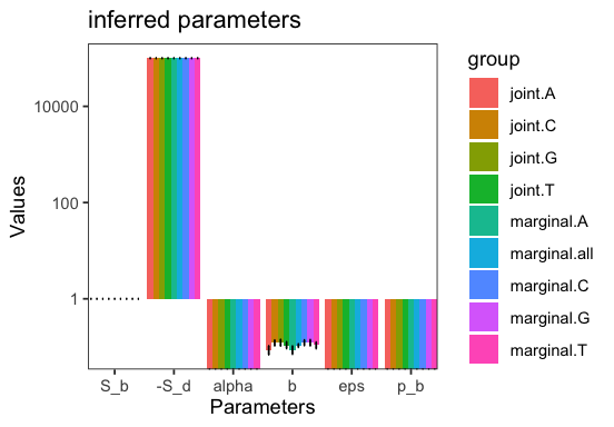
We see that S_d does not vary markedly across the jointly-inferred types and this is because it does not vary linearly along the arbitrary covariates we specified. Indeed, looking at the mean over all bootstraps for our covariate we see that it is close to 0. Note that covariates are named c0, c1, etc. by default.

mean(inf$bootstraps[['A.c0']])

1.06588538782984e-05

Model comparison

We can perform a likelihood ratio test to see whether including the covariates produces a significantly better fit than simply sharing the parameter in question among the types (cf. perform_lrt_covariates()).

joint_inference$perform_lrt_covariates(inf)

0.999991862224554

As expected, the specified covariates do not improve the fit significantly.