DFE inference#
Estimating the deleterious DFE#
A short overview of basic DFE inference and bootstrapping is available in the quickstart guide. DFE inference requires one neutral and one selected SFS. In this example we use the bundled Betula pendula (silver birch) data. By default, bootstrapping is performed automatically, and the inference estimates only the deleterious component of the DFE using GammaExpParametrization.
library(fastdfe)
fd <- load_fastdfe()
sfs_neut <- fd$Spectrum(c(177130, 997, 441, 228, 156, 117, 114, 83, 105, 109, 0))
sfs_sel <- fd$Spectrum(c(797939, 1329, 499, 265, 162, 104, 117, 90, 94, 119, 0))
# create inference object
inf <- fd$BaseInference(
sfs_neut = sfs_neut,
sfs_sel = sfs_sel
)
# run inference
sfs_modelled <- inf$run()
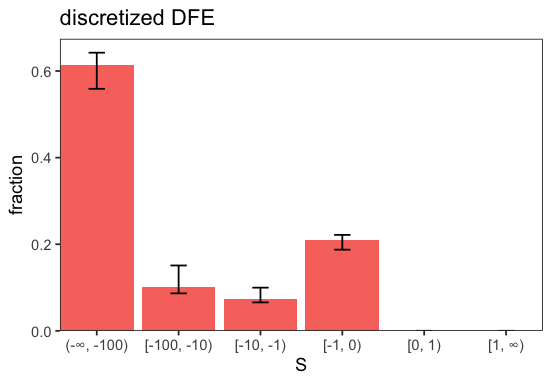
p <- inf$plot_discretized();
INFO:BaseInference: No divergence counts provided, inferring from polymorphism only.
INFO:Discretization: Precomputing semidominant DFE-SFS transformation using midpoint integration.
Discretization>Precomputing: 100%|██████████| 9/9 [00:00<00:00, 17.43it/s]
INFO:Optimization: Optimizing 2 parameters: [all.S_d, all.b].
BaseInference>Performing inference: 100%|██████████| 10/10 [00:00<00:00, 72.28it/s]
INFO:BaseInference: Inference results: {all.S_d: -3.389e+04 ± 3.9, all.b: 0.1305 ± 1.6e-06, all.p_b: 0 ± 0, all.S_b: 1 ± 0, all.eps: 0 ± 0, all.h: 0.5 ± 0, likelihood: -35.44 ± 4.1e-09} (best_run ± std_across_runs)
BaseInference>Bootstrapping (2 runs each): 100%|██████████| 100/100 [00:02<00:00, 46.71it/s]
INFO:BaseInference: Bootstrap summary: {all.S_d: -5.482e+04 ± 3.9e+04, all.b: 0.1331 ± 0.022, all.p_b: 0 ± 0, all.S_b: 1 ± 0, all.eps: 0 ± 0, all.h: 0.5 ± 0, likelihood: -42.9 ± 5.9, i_best_run: 0.47 ± 0.5, likelihoods_std: 0.003011 ± 0.022} (mean ± std)
It is always good practice to check the variability of estimates across optimization runs to ensure stability. Here, both the standard deviations across initial runs and across runs within each bootstrap sample are low, indicating stable estimates. Individual runs and bootstrap results can be inspected in the corresponding dataframes (cf. runs and bootstraps).
inf$runs[sapply(inf$runs, is.numeric)]
| all.S_d | all.b | all.p_b | all.S_b | all.eps | all.h | likelihood |
|---|---|---|---|---|---|---|
| <dbl> | <dbl> | <dbl> | <dbl> | <dbl> | <dbl> | <dbl> |
| -33901.43 | 0.1305413 | 0 | 1 | 0 | 0.5 | -35.43797 |
| -33892.20 | 0.1305452 | 0 | 1 | 0 | 0.5 | -35.43797 |
| -33892.13 | 0.1305452 | 0 | 1 | 0 | 0.5 | -35.43797 |
| -33895.01 | 0.1305440 | 0 | 1 | 0 | 0.5 | -35.43797 |
| -33892.73 | 0.1305449 | 0 | 1 | 0 | 0.5 | -35.43797 |
| -33900.32 | 0.1305418 | 0 | 1 | 0 | 0.5 | -35.43797 |
| -33889.39 | 0.1305463 | 0 | 1 | 0 | 0.5 | -35.43797 |
| -33897.77 | 0.1305428 | 0 | 1 | 0 | 0.5 | -35.43797 |
| -33892.25 | 0.1305451 | 0 | 1 | 0 | 0.5 | -35.43797 |
| -33895.27 | 0.1305439 | 0 | 1 | 0 | 0.5 | -35.43797 |
head(inf$bootstraps[sapply(inf$bootstraps, is.numeric)], 10)
| S_d | b | p_b | S_b | eps | h | likelihood | i_best_run | likelihoods_std | alpha | omega | omega_a | |
|---|---|---|---|---|---|---|---|---|---|---|---|---|
| <dbl> | <dbl> | <dbl> | <dbl> | <dbl> | <dbl> | <dbl> | <dbl> | <dbl> | <dbl> | <dbl> | <dbl> | |
| 1 | -100000.000 | 0.1152711 | 0 | 1 | 0 | 0.5 | -48.66672 | 0 | 7.105427e-13 | 0 | 0.2207236 | 0 |
| 2 | -23098.869 | 0.1327676 | 0 | 1 | 0 | 0.5 | -39.45439 | 1 | 1.097931e-10 | 0 | 0.2171733 | 0 |
| 3 | -30895.473 | 0.1265256 | 0 | 1 | 0 | 0.5 | -44.11652 | 1 | 3.521734e-10 | 0 | 0.2235578 | 0 |
| 4 | -100000.000 | 0.1170411 | 0 | 1 | 0 | 0.5 | -40.33266 | 1 | 3.077001e-02 | 0 | 0.2160429 | 0 |
| 5 | -27264.682 | 0.1347712 | 0 | 1 | 0 | 0.5 | -38.64248 | 0 | 4.202718e-10 | 0 | 0.2079502 | 0 |
| 6 | -100000.000 | 0.1150590 | 0 | 1 | 0 | 0.5 | -36.25929 | 1 | 1.250555e-12 | 0 | 0.2212916 | 0 |
| 7 | -16452.370 | 0.1420238 | 0 | 1 | 0 | 0.5 | -40.44355 | 0 | 4.688729e-10 | 0 | 0.2068260 | 0 |
| 8 | -5995.119 | 0.1644742 | 0 | 1 | 0 | 0.5 | -43.46204 | 0 | 3.181157e-09 | 0 | 0.1949254 | 0 |
| 9 | -2350.232 | 0.1879433 | 0 | 1 | 0 | 0.5 | -38.71198 | 1 | 3.382183e-12 | 0 | 0.1886620 | 0 |
| 10 | -18058.854 | 0.1452622 | 0 | 1 | 0 | 0.5 | -39.21888 | 1 | 3.620926e-11 | 0 | 0.1974813 | 0 |
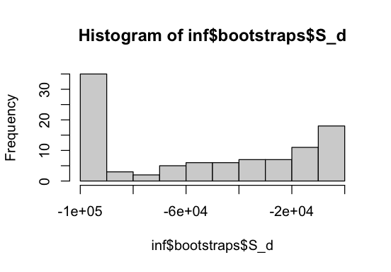
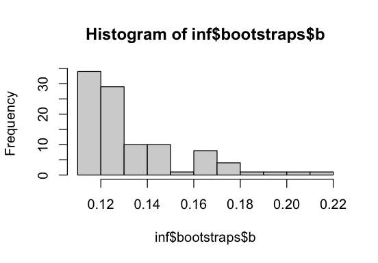
We can also plot the parameter distributions across bootstrap samples to visualize uncertainty. We see that the mean strength of deleterious selection S_d often reaches the lower bounds of -1e5. Perhaps a different DFE parameterization or a more complex DFE model would be more appropriate here. It should also be noted that the spectra used in this example are far from exemplary, as they contain few SNPs and have a small sample size.
hist(inf$bootstraps$S_d); hist(inf$bootstraps$b)
We can also inspect how parameters covary.
plot(abs(inf$bootstraps$S_d), inf$bootstraps$b, log="x")

We observe a slight dependence between the mean S_d and the shape parameter b of GammaExpParametrization. This is because a large fraction of moderately deleterious mutations and a smaller fraction of strongly deleterious mutations can leave a similar signal in the SFS. Spectra with larger sample sizes might facilitate disentangling the two.
Estimating beneficial effects#
Parameters can be held fixed during maximum-likelihood optimization, and this was already done internally in the example above. By default, fastdfe infers only the deleterious DFE, fixes the ancestral-allele misidentification rate eps, and assumes semi-dominant mutations (h = 0.5) (see fixed_params). Here, we estimate the full DFE, allowing for beneficial mutations by letting the parameters S_b and p_b of GammaExpParametrization vary, while eps and h remain fixed. The fixed parameters are wrapped in a dictionary under the key all, meaning these settings apply to all SFS types, which matters when running joint inference (cf. JointInference).
# create inference object
inf <- fd$BaseInference(
    sfs_neut = sfs_neut,
    sfs_sel = sfs_sel,
    fixed_params = list(all = list(eps = 0, h = 0.5))
)

# run inference
sfs_modelled <- inf$run()

p <- inf$plot_discretized();
INFO:BaseInference: No divergence counts provided, inferring from polymorphism only.
INFO:Discretization: Precomputing semidominant DFE-SFS transformation using midpoint integration.
Discretization>Precomputing: 100%|██████████| 9/9 [00:00<00:00, 17.28it/s]
INFO:Optimization: Optimizing 4 parameters: [all.S_d, all.p_b, all.b, all.S_b].
BaseInference>Performing inference: 100%|██████████| 10/10 [00:00<00:00, 18.57it/s]
WARNING:Optimization: The MLE estimate is close to the upper bound for {all.S_b: (0.0001, 100, 100)} and lower bound for {all.p_b: (0, 0.0043678413, 0.5)} [(lower, value, upper)], but this might be nothing to worry about.
INFO:BaseInference: Inference results: {all.S_d: -9823 ± 4.3e+03, all.b: 0.1549 ± 0.13, all.p_b: 0.004368 ± 0.091, all.S_b: 100 ± 52, all.eps: 0 ± 0, all.h: 0.5 ± 0, likelihood: -34.73 ± 0.24} (best_run ± std_across_runs)
BaseInference>Bootstrapping (2 runs each): 100%|██████████| 100/100 [00:07<00:00, 12.79it/s]
INFO:BaseInference: Bootstrap summary: {all.S_d: -2.191e+04 ± 3.4e+04, all.b: 0.7373 ± 2.1, all.p_b: 0.06208 ± 0.087, all.S_b: 57.97 ± 49, all.eps: 0 ± 0, all.h: 0.5 ± 0, likelihood: -40.92 ± 5.8, i_best_run: 0.39 ± 0.49, likelihoods_std: 0.3554 ± 0.65} (mean ± std)

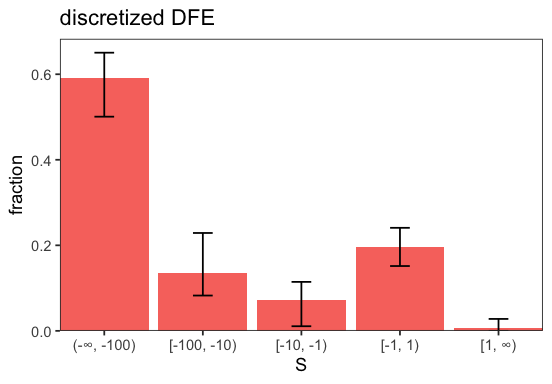
The inferred full DFE shows substantial uncertainty, which is expected with a small sample and few SNPs. This is most pronounced for the [-1, 0] and [0, 1] bins, where many mutations are effectively neutral and provide little signal. Adjusting the discretization intervals can help reveal the structure more clearly (cf. plot_discretized()).
p <- inf$plot_discretized(intervals = c(-Inf, -100, -10, -1, 1, Inf));
Divergence counts#
Besides polymorphism, fastdfe can incorporate divergence counts — the number of fixed differences (substitutions) to an outgroup — into the likelihood, much like polydfe. The last entry of an SFS is the fixed-derived (divergence) class. To make use of divergence, you additionally pass the divergence target sizes n_sites_div_neut and n_sites_div_sel to the inference — the number of mutational target sites over which divergence was counted, which may differ from the polymorphism target size.
When both spectra carry a separate divergence target size, divergence is included in the likelihood automatically (include_divergence = TRUE by default; see include_divergence). The selected divergence then helps constrain the beneficial part of the DFE, and \(\alpha\), the proportion of beneficial substitutions, can be estimated McDonald–Kreitman style from the observed divergence. The estimator used by get_alpha() follows the inference mode, but can be switched explicitly via its use_divergence argument.
# the SFS runs from the monomorphic (ancestral) class through the polymorphic bins to the
# fixed-derived (divergence) class in the last entry. The divergence target sizes are
# given to the inference (n_sites_div_neut / n_sites_div_sel), not to the spectra
sfs_neut <- fd$Spectrum(c(171150, 997, 441, 228, 156, 117, 114, 83, 105, 109, 6500))
sfs_sel <- fd$Spectrum(c(793221, 1329, 499, 265, 162, 104, 117, 90, 94, 119, 14000))

# specifying the divergence target sizes opts divergence into the likelihood
inf <- fd$BaseInference(
    sfs_neut = sfs_neut,
    sfs_sel = sfs_sel,
    n_sites_div_neut = 180000,
    n_sites_div_sel = 810000,
    fixed_params = list(all = list(eps = 0, h = 0.5))
)
sfs_modelled <- inf$run()

# alpha using divergence (McDonald-Kreitman style) vs. from polymorphism alone
cat('alpha (with divergence):  ', inf$get_alpha(), '\n')
cat('alpha (polymorphism only):', inf$get_alpha(use_divergence = FALSE), '\n')

# the rate of non-synonymous over synonymous substitutions (omega = dN/dS) and its
# adaptive component (omega_a = alpha * omega) are reported analogously
cat('omega:  ', inf$get_omega(), '\n')
cat('omega_a:', inf$get_omega_a(), '\n')
alpha (with divergence):   0.6614585
alpha (polymorphism only): 0.5940308
omega:   0.4786325
omega_a: 0.3165955
INFO:BaseInference: Using divergence counts in the likelihood.
INFO:Discretization: Precomputing semidominant DFE-SFS transformation using midpoint integration.
Discretization>Precomputing: 100%|██████████| 9/9 [00:00<00:00, 17.21it/s]
INFO:Optimization: Optimizing 4 parameters: [all.S_d, all.p_b, all.b, all.S_b].
BaseInference>Performing inference: 100%|██████████| 10/10 [00:02<00:00,  4.88it/s]
WARNING:Optimization: The MLE estimate is close to the upper bound for {} and lower bound for {all.p_b: (0, 0.0044950944, 0.5)} [(lower, value, upper)], but this might be nothing to worry about.
INFO:BaseInference: Inference results: {all.S_d: -1.059e+04 ± 2.8e+04, all.b: 0.1545 ± 3.1, all.p_b: 0.004495 ± 0.13, all.S_b: 63.22 ± 24, all.eps: 0 ± 0, all.h: 0.5 ± 0, likelihood: -45.75 ± 1.6e+02} (best_run ± std_across_runs)
BaseInference>Bootstrapping (2 runs each): 100%|██████████| 100/100 [00:27<00:00,  3.63it/s]
INFO:BaseInference: Bootstrap summary: {all.S_d: -2.606e+04 ± 3.6e+04, all.b: 0.1642 ± 0.038, all.p_b: 0.007739 ± 0.0075, all.S_b: 61.74 ± 32, all.eps: 0 ± 0, all.h: 0.5 ± 0, likelihood: -52.5 ± 5.3, i_best_run: 0.48 ± 0.5, likelihoods_std: 15.75 ± 51} (mean ± std)
Ancestral-allele misidentification#
We can also adjust for ancestral-allele misidentification by letting parameter eps vary. eps is the probability that an allele is misidentified as derived when it is actually ancestral, and vice versa (cf. misidentify()). This can correct biases to the SFS caused by mis-polarization, but eps is somewhat difficult to interpret because it is applied simultaneously to both the neutral and selected SFS. In addition, eps assumes the fraction of ancestral misidentification to be constant across site classes, but in practise errors may differ across classes. Nevertheless, below, we infer the full DFE while allowing eps to vary.
inf <- fd$BaseInference(
    sfs_neut = sfs_neut,
    sfs_sel = sfs_sel,
    fixed_params = list(all = list(h=0.5))
)

sfs_modelled <- inf$run()
INFO:BaseInference: No divergence counts provided, inferring from polymorphism only.
INFO:Discretization: Precomputing semidominant DFE-SFS transformation using midpoint integration.
Discretization>Precomputing: 100%|██████████| 9/9 [00:00<00:00, 17.14it/s]
INFO:Optimization: Optimizing 5 parameters: [all.p_b, all.S_b, all.S_d, all.eps, all.b].
BaseInference>Performing inference: 100%|██████████| 10/10 [00:00<00:00, 13.99it/s]
WARNING:Optimization: The MLE estimate is close to the upper bound for {} and lower bound for {all.p_b: (0, 0, 0.5)} [(lower, value, upper)], but this might be nothing to worry about.
INFO:BaseInference: Inference results: {all.S_d: -1.064e+04 ± 3.6e+03, all.b: 0.1508 ± 0.0036, all.p_b: 0 ± 0.0018, all.S_b: 0.0001247 ± 0.051, all.eps: 0.006854 ± 0.00084, all.h: 0.5 ± 0, likelihood: -34.63 ± 0.052} (best_run ± std_across_runs)
BaseInference>Bootstrapping (2 runs each): 100%|██████████| 100/100 [00:10<00:00,  9.41it/s]
INFO:BaseInference: Bootstrap summary: {all.S_d: -2.086e+04 ± 3.4e+04, all.b: 0.9853 ± 2.5, all.p_b: 0.08495 ± 0.092, all.S_b: 0.02081 ± 0.14, all.eps: 0.006606 ± 0.0073, all.h: 0.5 ± 0, likelihood: -40.4 ± 5, i_best_run: 0.47 ± 0.5, likelihoods_std: 0.02819 ± 0.097} (mean ± std)
hist(inf$bootstraps$eps)
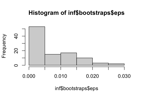
eps is estimated to be rather low, indicating that ancestral-allele misidentification is not a major issue in this dataset, or, at least, that including it that does not significantly improve the model fit. We can also check this in a more principled way by performing a likelihood-ratio test as done below.
Nested model comparison#
We can automatically check for the significance of include ancestral-allele misidentification and beneficial fitness affects using likelihood ratio tests. This is done with plot_nested_models(). The LRTs are performed by comparing the likelihood of the inferred DFE to the likelihood of a nested model where some parameters are held fixed. Alternatively, we can use compare_nested() to directly compare two nested models.
# set logging level to warning to avoid cluttering
fd$logger$setLevel('WARNING')

p <- inf$plot_nested_models();

fd$logger$setLevel('INFO')
BaseInference>Performing inference: 100%|██████████| 10/10 [00:00<00:00, 15.35it/s]
WARNING:Optimization: The MLE estimate is close to the upper bound for {all.S_b: (0.0001, 100, 100)} and lower bound for {all.p_b: (0, 0.0043298919, 0.5)} [(lower, value, upper)], but this might be nothing to worry about.
BaseInference>Performing inference: 100%|██████████| 10/10 [00:00<00:00, 14.20it/s]
WARNING:Optimization: The MLE estimate is close to the upper bound for {} and lower bound for {all.p_b: (0, 0, 0.5)} [(lower, value, upper)], but this might be nothing to worry about.
BaseInference>Performing inference: 100%|██████████| 10/10 [00:00<00:00, 67.93it/s]
BaseInference>Performing inference: 100%|██████████| 10/10 [00:00<00:00, 47.31it/s]
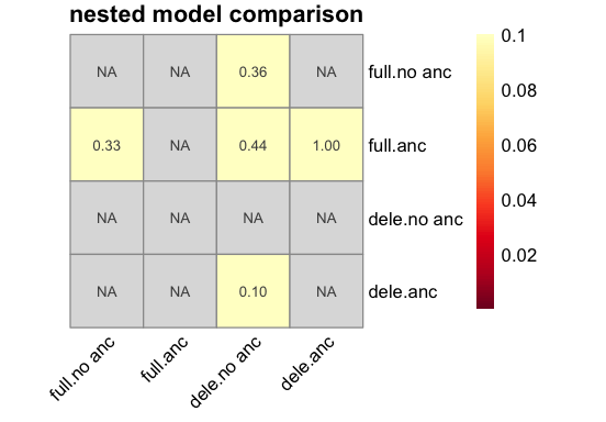
Including ancestral allele misidentification or beneficial mutations does not appear to improve the fit significantly.
Dominance effects#
By default, fastdfe assumes semi-dominance (h = 0.5), which is more or less appropriate depending on the organism and type of mutations considered. We can change the dominance coefficient to a different value of h if we believe this is more appropriate. However, in practise, h often depends on the strength of selection, with more deleterious mutations being more recessive. To model this, we can specify a callback function that returns the dominance coefficient as a function of the selection coefficient S = 4Ne.
In the example below, we use an exponential decay: h is about 0.4 for neutral mutations and approaches 0 for strongly deleterious ones. The callback also receives h itself, allowing the dominance function to be parametrized and optimized; for simplicity, this parameter is still called h. Its bounds can be set via bounds.
inf <- fd$BaseInference(
    sfs_neut = sfs_neut,
    sfs_sel = sfs_sel,
    fixed_params = list(all = list(eps = 0, h = 0, p_b = 0, S_b = 1)),
    h_callback=function(h, S) { 0.4 * exp(-0.1 * abs(S)) }
)

sfs_modelled <- inf$run()
INFO:BaseInference: No divergence counts provided, inferring from polymorphism only.
INFO:Discretization: Precomputing DFE-SFS transformation for fixed dominance coefficients.
Discretization>Precomputing: 100%|██████████| 1809/1809 [00:20<00:00, 87.74it/s]
INFO:Optimization: Optimizing 2 parameters: [all.S_d, all.b].
BaseInference>Performing inference: 100%|██████████| 10/10 [00:00<00:00, 117.67it/s]
WARNING:Optimization: The MLE estimate is close to the upper bound for {} and lower bound for {all.S_d: (-100000, -100000, -0.01)} [(lower, value, upper)], but this might be nothing to worry about.
WARNING:BaseInference: The L1 residual comparing the modelled and observed SFS is rather large: `norm(sfs_modelled - sfs_observed, 1) / sfs_observed` = 0.159. This may indicate that the model does not fit the data well.
INFO:BaseInference: Inference results: {all.S_d: -1e+05 ± 0, all.b: 0.1411 ± 2.6e-09, all.p_b: 0 ± 0, all.S_b: 1 ± 0, all.eps: 0 ± 0, all.h: 0 ± 0, likelihood: -75.43 ± 1.2e-12} (best_run ± std_across_runs)
BaseInference>Bootstrapping (2 runs each): 100%|██████████| 100/100 [00:01<00:00, 79.51it/s]
INFO:BaseInference: Bootstrap summary: {all.S_d: -1e+05 ± 0, all.b: 0.1405 ± 0.0034, all.p_b: 0 ± 0, all.S_b: 1 ± 0, all.eps: 0 ± 0, all.h: 0 ± 0, likelihood: -84.58 ± 15, i_best_run: 0.45 ± 0.5, likelihoods_std: 1.861 ± 18} (mean ± std)
Let’s compare the inferred DFE under this dominance relationship to that of the default semi-dominant model.
inf2 <- fd$BaseInference(
    sfs_neut = sfs_neut,
    sfs_sel = sfs_sel,
    fixed_params = list(all = list(eps = 0, h = 0.5, p_b = 0, S_b = 1))
)

sfs_modelled <- inf2$run()
INFO:BaseInference: No divergence counts provided, inferring from polymorphism only.
INFO:Discretization: Precomputing semidominant DFE-SFS transformation using midpoint integration.
Discretization>Precomputing: 100%|██████████| 9/9 [00:00<00:00, 17.19it/s]
INFO:Optimization: Optimizing 2 parameters: [all.S_d, all.b].
BaseInference>Performing inference: 100%|██████████| 10/10 [00:00<00:00, 76.53it/s]
INFO:BaseInference: Inference results: {all.S_d: -3.621e+04 ± 3.8, all.b: 0.1305 ± 1.5e-06, all.p_b: 0 ± 0, all.S_b: 1 ± 0, all.eps: 0 ± 0, all.h: 0.5 ± 0, likelihood: -35.44 ± 4.6e-09} (best_run ± std_across_runs)
BaseInference>Bootstrapping (2 runs each): 100%|██████████| 100/100 [00:02<00:00, 46.14it/s]
INFO:BaseInference: Bootstrap summary: {all.S_d: -5.203e+04 ± 4.1e+04, all.b: 0.1346 ± 0.019, all.p_b: 0 ± 0, all.S_b: 1 ± 0, all.eps: 0 ± 0, all.h: 0.5 ± 0, likelihood: -43.02 ± 5.9, i_best_run: 0.41 ± 0.49, likelihoods_std: 0.007273 ± 0.057} (mean ± std)
p <- fd$DFE$plot_many(c(inf$get_dfe(), inf2$get_dfe()), labels=c('partly recessive', 'h=0.5'))
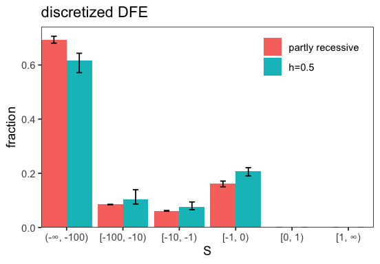
We see that assuming mutations are partly recessive leads to a more deleterious inferred DFE since stronger selection is necessary to remove a similar amount of recessive mutations.
We can also let h vary when inferring the DFE (cf. the simulation guide).
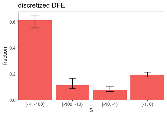
Folded inference#
To infer the DFE from a folded SFS, simply pass folded spectra to BaseInference. Folded inference is performed whenever the spectra are folded, i.e., when all entries where the derived allele is the major allele are zero. Folded spectra contain little information on beneficial mutations so we only infer the deleterious part of the DFE here.
# create inference object
inf <- fd$BaseInference(
    sfs_neut = sfs_neut$fold(),
    sfs_sel = sfs_sel$fold()
)

# run inference
sfs_modelled <- inf$run()

p <- inf$plot_discretized(intervals = c(-Inf, -100, -10, -1, 0));
INFO:BaseInference: No divergence counts provided, inferring from polymorphism only.
INFO:Discretization: Precomputing semidominant DFE-SFS transformation using midpoint integration.
Discretization>Precomputing: 100%|██████████| 9/9 [00:00<00:00, 17.02it/s]
INFO:Optimization: Optimizing 2 parameters: [all.S_d, all.b].
BaseInference>Performing inference: 100%|██████████| 10/10 [00:00<00:00, 64.17it/s]
INFO:BaseInference: Inference results: {all.S_d: -1.654e+04 ± 0.87, all.b: 0.1464 ± 9.4e-07, all.p_b: 0 ± 0, all.S_b: 1 ± 0, all.eps: 0 ± 0, all.h: 0.5 ± 0, likelihood: -21.58 ± 1.3e-09} (best_run ± std_across_runs)
BaseInference>Bootstrapping (2 runs each): 100%|██████████| 100/100 [00:02<00:00, 41.65it/s]
INFO:BaseInference: Bootstrap summary: {all.S_d: -3.778e+04 ± 3.9e+04, all.b: 0.1488 ± 0.027, all.p_b: 0 ± 0, all.S_b: 1 ± 0, all.eps: 0 ± 0, all.h: 0.5 ± 0, likelihood: -25.08 ± 4.2, i_best_run: 0.48 ± 0.5, likelihoods_std: 8.82e-10 ± 1.5e-09} (mean ± std)
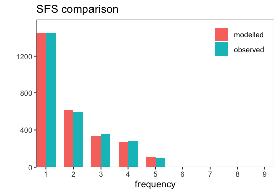
p <- inf$plot_sfs_comparison();
Serialization#
Inference objects can be serialized to JSON files for later use (cf. to_file()).
# save the inference object to a file
# unserialize with BaseInference$from_file
inf$to_file("serialized.json")

# we can also save a short summary to fa ile
inf$get_summary()$to_file("summary.json")
Joint inference#
fastdfe supports joint inference of several SFS types, where any parameters can be shared between types. In this example, we create a JointInference object with two types, where we share eps, the rate of ancestral misidentification and S_d, the mean selection coefficient for deleterious mutations (cf. GammaExpParametrization). For more complex stratifications, see the Parser) module.
# neutral SFS for two types
sfs_neut <- fd$Spectra(list(
    pendula = c(177130, 997, 441, 228, 156, 117, 114, 83, 105, 109, 0),
    pubescens = c(172528, 3612, 1359, 790, 584, 427, 325, 234, 166, 76, 0)
))

# selected SFS for two types
sfs_sel <- fd$Spectra(list(
    pendula = c(797939, 1329, 499, 265, 162, 104, 117, 90, 94, 119, 0),
    pubescens = c(791106, 5326, 1741, 1005, 756, 546, 416, 294, 177, 104, 0)
))

# create inference object
inf <- fd$JointInference(
    sfs_neut = sfs_neut,
    sfs_sel = sfs_sel,
    shared_params = list(fd$SharedParams(types = c("pendula", "pubescens"), params = list("S_d")))
)

# run inference
sfs_modelled <- inf$run()
INFO:JointInference: No divergence counts provided, inferring from polymorphism only.
INFO:JointInference: Using shared parameters [SharedParams(params=['S_d'], types=['pendula', 'pubescens'])].
INFO:JointInference: Including covariates: {}.
INFO:BaseInference: No divergence counts provided, inferring from polymorphism only.
INFO:BaseInference: No divergence counts provided, inferring from polymorphism only.
INFO:BaseInference: No divergence counts provided, inferring from polymorphism only.
INFO:BaseInference: No divergence counts provided, inferring from polymorphism only.
INFO:BaseInference: No divergence counts provided, inferring from polymorphism only.
INFO:JointInference: Running marginal inference for type 'all'.
INFO:Discretization: Precomputing semidominant DFE-SFS transformation using midpoint integration.
Discretization>Precomputing: 100%|██████████| 9/9 [00:00<00:00, 17.30it/s]
INFO:Optimization: Optimizing 2 parameters: [all.S_d, all.b].
BaseInference>Performing inference: 100%|██████████| 10/10 [00:00<00:00, 80.79it/s]
WARNING:Optimization: The MLE estimate is close to the upper bound for {} and lower bound for {all.S_d: (-100000, -100000, -0.01)} [(lower, value, upper)], but this might be nothing to worry about.
INFO:BaseInference: Inference results: {all.S_d: -1e+05 ± 5.7e+03, all.b: 0.1066 ± 0.00064, all.p_b: 0 ± 0, all.S_b: 1 ± 0, all.eps: 0 ± 0, all.h: 0.5 ± 0, likelihood: -45.09 ± 0.04} (best_run ± std_across_runs)
INFO:JointInference: Running marginal inferences for types ['pendula', 'pubescens'].
INFO:JointInference: Running marginal inference for type 'pendula'.
INFO:Optimization: Optimizing 2 parameters: [all.S_d, all.b].
BaseInference>Performing inference: 100%|██████████| 10/10 [00:00<00:00, 71.44it/s]
INFO:BaseInference: Inference results: {all.S_d: -3.389e+04 ± 3.2, all.b: 0.1305 ± 1.3e-06, all.p_b: 0 ± 0, all.S_b: 1 ± 0, all.eps: 0 ± 0, all.h: 0.5 ± 0, likelihood: -35.44 ± 2.8e-09} (best_run ± std_across_runs)
INFO:JointInference: Running marginal inference for type 'pubescens'.
INFO:Optimization: Optimizing 2 parameters: [all.S_d, all.b].
BaseInference>Performing inference: 100%|██████████| 10/10 [00:00<00:00, 81.13it/s]
WARNING:Optimization: The MLE estimate is close to the upper bound for {} and lower bound for {all.S_d: (-100000, -100000, -0.01)} [(lower, value, upper)], but this might be nothing to worry about.
INFO:BaseInference: Inference results: {all.S_d: -1e+05 ± 0, all.b: 0.1035 ± 2.3e-09, all.p_b: 0 ± 0, all.S_b: 1 ± 0, all.eps: 0 ± 0, all.h: 0.5 ± 0, likelihood: -43.81 ± 7.7e-12} (best_run ± std_across_runs)
INFO:JointInference: Running joint inference for types ['pendula', 'pubescens'].
INFO:Optimization: Optimizing 3 parameters: [pendula:pubescens.S_d, pubescens.b, pendula.b].
JointInference>Performing joint inference: 100%|██████████| 10/10 [00:00<00:00, 25.41it/s]
WARNING:Optimization: The MLE estimate is close to the upper bound for {} and lower bound for {pendula:pubescens.S_d: (-100000, -100000, -0.01)} [(lower, value, upper)], but this might be nothing to worry about.
INFO:JointInference: Inference results: {pendula.b: 0.1168 ± 0.00058, pendula.p_b: 0 ± 0, pendula.S_b: 1 ± 0, pendula.eps: 0 ± 0, pendula.h: 0.5 ± 0, pubescens.b: 0.1035 ± 0.00052, pubescens.p_b: 0 ± 0, pubescens.S_b: 1 ± 0, pubescens.eps: 0 ± 0, pubescens.h: 0.5 ± 0, pendula:pubescens.S_d: -1e+05 ± 4.8e+03, likelihood: -79.47 ± 0.049} (best_run ± std_across_runs)
INFO:JointInference: Bootstrapping type 'all'.
BaseInference>Bootstrapping 'all' (2 runs each): 100%|██████████| 100/100 [00:01<00:00, 54.34it/s]
INFO:BaseInference: Bootstrap summary: {all.S_d: -8.66e+04 ± 2.7e+04, all.b: 0.1094 ± 0.0073, all.p_b: 0 ± 0, all.S_b: 1 ± 0, all.eps: 0 ± 0, all.h: 0.5 ± 0, likelihood: -54 ± 7.5, i_best_run: 0.48 ± 0.5, likelihoods_std: 0.003665 ± 0.033} (mean ± std)
INFO:JointInference: Bootstrapping type 'pendula'.
BaseInference>Bootstrapping 'pendula' (2 runs each): 100%|██████████| 100/100 [00:02<00:00, 46.70it/s]
INFO:BaseInference: Bootstrap summary: {all.S_d: -5.482e+04 ± 3.9e+04, all.b: 0.1331 ± 0.022, all.p_b: 0 ± 0, all.S_b: 1 ± 0, all.eps: 0 ± 0, all.h: 0.5 ± 0, likelihood: -42.9 ± 5.9, i_best_run: 0.47 ± 0.5, likelihoods_std: 0.003011 ± 0.022} (mean ± std)
INFO:JointInference: Bootstrapping type 'pubescens'.
BaseInference>Bootstrapping 'pubescens' (2 runs each): 100%|██████████| 100/100 [00:01<00:00, 57.55it/s]
INFO:BaseInference: Bootstrap summary: {all.S_d: -9.267e+04 ± 2.1e+04, all.b: 0.1049 ± 0.0055, all.p_b: 0 ± 0, all.S_b: 1 ± 0, all.eps: 0 ± 0, all.h: 0.5 ± 0, likelihood: -53.15 ± 7.6, i_best_run: 0.42 ± 0.5, likelihoods_std: 0.0007327 ± 0.0073} (mean ± std)
JointInference>Bootstrapping joint inference (2 runs each): 100%|██████████| 100/100 [00:05<00:00, 19.17it/s]
INFO:JointInference: Bootstrap summary: {pendula.b: 0.1199 ± 0.0069, pendula.p_b: 0 ± 0, pendula.S_b: 1 ± 0, pendula.eps: 0 ± 0, pendula.h: 0.5 ± 0, pendula.S_d: -8.715e+04 ± 2.5e+04, pubescens.b: 0.1058 ± 0.0059, pubescens.p_b: 0 ± 0, pubescens.S_b: 1 ± 0, pubescens.eps: 0 ± 0, pubescens.h: 0.5 ± 0, pubescens.S_d: -8.715e+04 ± 2.5e+04, likelihood: -96.89 ± 9.2, i_best_run: 0.59 ± 0.49, likelihoods_std: 6.774 ± 68} (mean ± std)
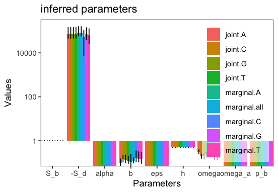
JointInference both runs the joint inference and marginal inference where each type is inferred separately. To see this better we can plot the inferred parameters for the different inference types.
p <- inf$plot_inferred_parameters();
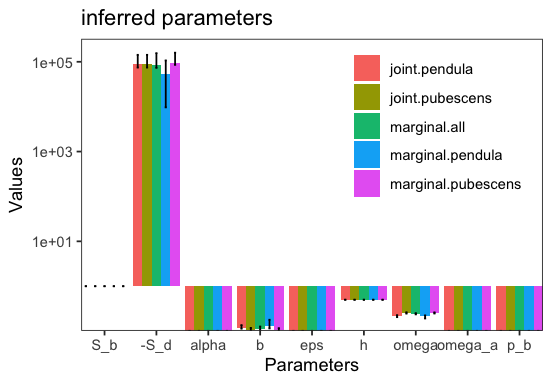
marginal.pendula and marginal.pubescens are the marginal inferences for the respective type. marginal.all is the marginal inference obtaining by adding up the spectra of all types. joint.pendula and join.pubescens are the joint inferences for the respective type. We can see that eps and S_d are indeed shared between the two. The parameter alpha in the plot denotes the proportion of beneficial non-synonymous substitutions. Each marginal inference is a BaseInference object itself and can be accessed via inf.marginal_inferences[type].
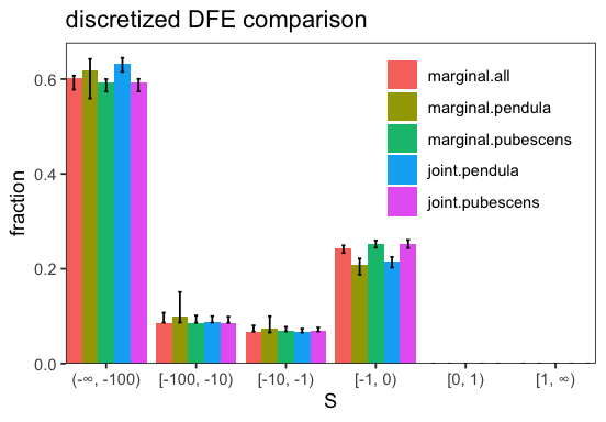
We can now also investigate to what extent the inferred DFEs differ:
p <- inf$plot_discretized();
Model comparison#
We can obtain information about the goodness of fit achieved by sharing the parameter by performing a likelihood ratio test (cf. perform_lrt_shared()). This compares the likelihood of the joint inference with the product of the marginal likelihoods.
inf$perform_lrt_shared()
INFO:JointInference: Simple model likelihood: -79.46612774561032, Complex model likelihood: -79.24883685478324, Total degrees of freedom: 1, Parameters at boundary: 0.
The test is not significant, indicating that the simpler model of sharing the parameters explains the data sufficiently well. Indeed, we do not observe a lot of differences between the inferred parameters of joint and the marginal inferences.
Covariates#
JointInference also supports the inclusion of covariates associates with the different SFS types. This provides more powerful model testing and reduces the number of parameters that need to be estimated for the joint inference. For a more interesting example we stratify the SFS of B. pendula by the sites’ reference base as is described in more detail in the sfsutils stratifications reference.
# instantiate parser
p <- fd$Parser(
n = 10,
vcf = paste0(
"https://github.com/Sendrowski/fastDFE/",
"blob/dev/resources/genome/betula/",
"all.polarized.deg.subset.200000.vcf.gz?raw=true"
),
stratifications = list(fd$DegeneracyStratification(), fd$AncestralBaseStratification())
)
# parse SFS
s <- p$parse()
# visualize spectra
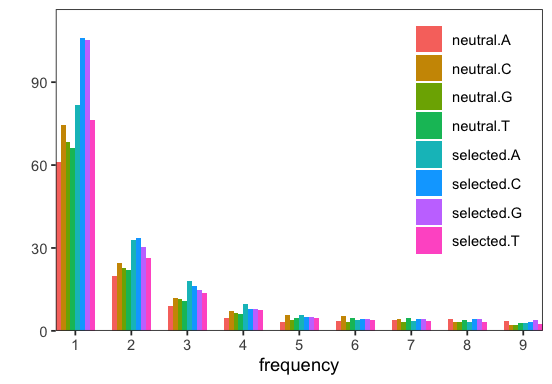
p <- s$plot();
INFO:Parser: Using stratification: [neutral, selected].[A, C, G, T].
INFO:Parser: Loading VCF file
INFO:FileHandler: Using cached file at /var/folders/n4/m5q2jgw91zv0tp1c4j9bh48m0000gn/T/011b01ee5cec.all.polarized.deg.subset.200000.vcf.gz
INFO:FileHandler: Using cached file at /var/folders/n4/m5q2jgw91zv0tp1c4j9bh48m0000gn/T/011b01ee5cec.all.polarized.deg.subset.200000.vcf.gz
Parser>Counting sites: 200000it [00:01, 143092.73it/s]
Parser>Processing sites: 100%|██████████| 200000/200000 [00:40<00:00, 4962.73it/s]
INFO:PolyAllelicFiltration: Filtered out 154 sites.
INFO:DegeneracyStratification: Number of sites with valid type: 64083
INFO:AncestralBaseStratification: Number of sites with valid type: 64083
INFO:Parser: Skipped 983 sites without ancestral allele information.
INFO:Parser: Included 64083 out of 200000 sites in total from the input.
We now create the inference object from the spectra. In this contrived example we make up some covariates that covary with S_d, the mean strength of negative selection. Covariates introduce a linear relationship by default but this can be modified by specifying a custom callback function (see Covariate).
# create inference object
inf <- fd$JointInference(
    sfs_neut = s$select('neutral.*')$merge_groups(1),
    sfs_sel = s$select('selected.*')$merge_groups(1),
    covariates = list(fd$Covariate(param = 'S_d', values = list(A = 1, C = 2, T = 3, G = 4))),
    n_runs = 50  # increase number of initial runs for stability
)

# run inference
sfs_modelled <- inf$run()
INFO:JointInference: No divergence counts provided, inferring from polymorphism only.
INFO:JointInference: Parameters ['S_d'] have covariates and thus need to be shared. Adding them to shared parameters.
INFO:JointInference: Using shared parameters [SharedParams(params=['S_d'], types=['A', 'C', 'G', 'T'])].
INFO:JointInference: Including covariates: {'c0': {'param': 'S_d', 'values': {'A': 1.0, 'C': 2.0, 'T': 3.0, 'G': 4.0}}}.
INFO:BaseInference: No divergence counts provided, inferring from polymorphism only.
INFO:BaseInference: No divergence counts provided, inferring from polymorphism only.
INFO:BaseInference: No divergence counts provided, inferring from polymorphism only.
INFO:BaseInference: No divergence counts provided, inferring from polymorphism only.
INFO:BaseInference: No divergence counts provided, inferring from polymorphism only.
INFO:BaseInference: No divergence counts provided, inferring from polymorphism only.
INFO:BaseInference: No divergence counts provided, inferring from polymorphism only.
INFO:BaseInference: No divergence counts provided, inferring from polymorphism only.
INFO:BaseInference: No divergence counts provided, inferring from polymorphism only.
INFO:JointInference: Running marginal inference for type 'all'.
INFO:Discretization: Precomputing semidominant DFE-SFS transformation using midpoint integration.
Discretization>Precomputing: 100%|██████████| 9/9 [00:00<00:00, 16.96it/s]
INFO:Optimization: Optimizing 2 parameters: [all.S_d, all.b].
BaseInference>Performing inference: 100%|██████████| 50/50 [00:00<00:00, 90.40it/s]
WARNING:Optimization: The MLE estimate is close to the upper bound for {} and lower bound for {all.S_d: (-100000, -100000, -0.01)} [(lower, value, upper)], but this might be nothing to worry about.
INFO:BaseInference: Inference results: {all.S_d: -1e+05 ± 6.1e+03, all.b: 0.1069 ± 0.0008, all.p_b: 0 ± 0, all.S_b: 1 ± 0, all.eps: 0 ± 0, all.h: 0.5 ± 0, likelihood: -26.61 ± 0.017} (best_run ± std_across_runs)
INFO:JointInference: Running marginal inferences for types ['A', 'C', 'G', 'T'].
INFO:JointInference: Running marginal inference for type 'A'.
INFO:Optimization: Optimizing 2 parameters: [all.S_d, all.b].
BaseInference>Performing inference: 100%|██████████| 50/50 [00:00<00:00, 96.00it/s]
WARNING:Optimization: The MLE estimate is close to the upper bound for {} and lower bound for {all.S_d: (-100000, -100000, -0.01)} [(lower, value, upper)], but this might be nothing to worry about.
WARNING:BaseInference: The L1 residual comparing the modelled and observed SFS is rather large: `norm(sfs_modelled - sfs_observed, 1) / sfs_observed` = 0.200. This may indicate that the model does not fit the data well.
INFO:BaseInference: Inference results: {all.S_d: -1e+05 ± 0, all.b: 0.0857 ± 2.8e-08, all.p_b: 0 ± 0, all.S_b: 1 ± 0, all.eps: 0 ± 0, all.h: 0.5 ± 0, likelihood: -22.72 ± 4.8e-11} (best_run ± std_across_runs)
INFO:JointInference: Running marginal inference for type 'C'.
INFO:Optimization: Optimizing 2 parameters: [all.S_d, all.b].
BaseInference>Performing inference: 100%|██████████| 50/50 [00:00<00:00, 80.38it/s]
WARNING:Optimization: The MLE estimate is close to the upper bound for {} and lower bound for {all.S_d: (-100000, -100000, -0.01)} [(lower, value, upper)], but this might be nothing to worry about.
INFO:BaseInference: Inference results: {all.S_d: -1e+05 ± 2.7e+03, all.b: 0.1219 ± 0.00035, all.p_b: 0 ± 0, all.S_b: 1 ± 0, all.eps: 0 ± 0, all.h: 0.5 ± 0, likelihood: -19.47 ± 0.0001} (best_run ± std_across_runs)
INFO:JointInference: Running marginal inference for type 'G'.
INFO:Optimization: Optimizing 2 parameters: [all.S_d, all.b].
BaseInference>Performing inference: 100%|██████████| 50/50 [00:00<00:00, 93.90it/s]
WARNING:Optimization: The MLE estimate is close to the upper bound for {} and lower bound for {all.S_d: (-100000, -100000, -0.01)} [(lower, value, upper)], but this might be nothing to worry about.
INFO:BaseInference: Inference results: {all.S_d: -1e+05 ± 9.9e+03, all.b: 0.1221 ± 0.0018, all.p_b: 0 ± 0, all.S_b: 1 ± 0, all.eps: 0 ± 0, all.h: 0.5 ± 0, likelihood: -18.88 ± 0.0095} (best_run ± std_across_runs)
INFO:JointInference: Running marginal inference for type 'T'.
INFO:Optimization: Optimizing 2 parameters: [all.S_d, all.b].
BaseInference>Performing inference: 100%|██████████| 50/50 [00:00<00:00, 93.15it/s]
WARNING:Optimization: The MLE estimate is close to the upper bound for {} and lower bound for {all.S_d: (-100000, -100000, -0.01)} [(lower, value, upper)], but this might be nothing to worry about.
INFO:BaseInference: Inference results: {all.S_d: -1e+05 ± 6.3e+03, all.b: 0.1079 ± 0.00081, all.p_b: 0 ± 0, all.S_b: 1 ± 0, all.eps: 0 ± 0, all.h: 0.5 ± 0, likelihood: -18.44 ± 0.0027} (best_run ± std_across_runs)
INFO:JointInference: Running joint inference for types ['A', 'C', 'G', 'T'].
INFO:Optimization: Optimizing 6 parameters: [C.b, G.b, A:C:G:T.S_d, T.b, A.b, A:C:G:T.c0].
JointInference>Performing joint inference: 100%|██████████| 50/50 [00:04<00:00, 10.75it/s]
WARNING:Optimization: The MLE estimate is close to the upper bound for {} and lower bound for {A:C:G:T.S_d: (-100000, -100000, -0.01)} [(lower, value, upper)], but this might be nothing to worry about.
WARNING:JointInference: Numerical optimization did not terminate normally, so the result might be unreliable. Consider adjusting the optimization parameters (increasing `gtol` or `n_runs`) or decreasing the number of optimized parameters.
INFO:JointInference: Inference results: {A.b: 0.0857 ± 3.7, A.p_b: 0 ± 0, A.S_b: 1 ± 0, A.eps: 0 ± 0, A.h: 0.5 ± 0, C.b: 0.1219 ± 1.8, C.p_b: 0 ± 0, C.S_b: 1 ± 0, C.eps: 0 ± 0, C.h: 0.5 ± 0, G.b: 0.1221 ± 0.5, G.p_b: 0 ± 0, G.S_b: 1 ± 0, G.eps: 0 ± 0, G.h: 0.5 ± 0, T.b: 0.1079 ± 1.6, T.p_b: 0 ± 0, T.S_b: 1 ± 0, T.eps: 0 ± 0, T.h: 0.5 ± 0, A:C:G:T.S_d: -1e+05 ± 4.8e+04, A:C:G:T.c0: 0 ± 5.5e+03, likelihood: -79.5 ± 4.2e+02} (best_run ± std_across_runs)
WARNING:BaseInference: The L1 residual comparing the modelled and observed SFS is rather large: `norm(sfs_modelled - sfs_observed, 1) / sfs_observed` = 0.200. This may indicate that the model does not fit the data well.
INFO:JointInference: Bootstrapping type 'all'.
BaseInference>Bootstrapping 'all' (2 runs each): 100%|██████████| 100/100 [00:01<00:00, 58.02it/s]
INFO:BaseInference: Bootstrap summary: {all.S_d: -7.909e+04 ± 3.8e+04, all.b: 0.1159 ± 0.021, all.p_b: 0 ± 0, all.S_b: 1 ± 0, all.eps: 0 ± 0, all.h: 0.5 ± 0, likelihood: -34.83 ± 5, i_best_run: 0.51 ± 0.5, likelihoods_std: 0.0002111 ± 0.0017} (mean ± std)
INFO:JointInference: Bootstrapping type 'A'.
BaseInference>Bootstrapping 'A' (2 runs each): 100%|██████████| 100/100 [00:01<00:00, 57.24it/s]
INFO:BaseInference: Bootstrap summary: {all.S_d: -7.963e+04 ± 3.9e+04, all.b: 0.1064 ± 0.052, all.p_b: 0 ± 0, all.S_b: 1 ± 0, all.eps: 0 ± 0, all.h: 0.5 ± 0, likelihood: -89.3 ± 1.7e+02, i_best_run: 0.46 ± 0.5, likelihoods_std: 0.001599 ± 0.012} (mean ± std)
INFO:JointInference: Bootstrapping type 'C'.
BaseInference>Bootstrapping 'C' (2 runs each): 100%|██████████| 100/100 [00:01<00:00, 52.66it/s]
INFO:BaseInference: Bootstrap summary: {all.S_d: -5.36e+04 ± 4.7e+04, all.b: 0.1704 ± 0.084, all.p_b: 0 ± 0, all.S_b: 1 ± 0, all.eps: 0 ± 0, all.h: 0.5 ± 0, likelihood: -115.3 ± 1.9e+02, i_best_run: 0.47 ± 0.5, likelihoods_std: 0.06328 ± 0.46} (mean ± std)
INFO:JointInference: Bootstrapping type 'G'.
BaseInference>Bootstrapping 'G' (2 runs each): 100%|██████████| 100/100 [00:01<00:00, 57.52it/s]
INFO:BaseInference: Bootstrap summary: {all.S_d: -6.976e+04 ± 4.3e+04, all.b: 0.1514 ± 0.061, all.p_b: 0 ± 0, all.S_b: 1 ± 0, all.eps: 0 ± 0, all.h: 0.5 ± 0, likelihood: -157.3 ± 2.4e+02, i_best_run: 0.46 ± 0.5, likelihoods_std: 0.01676 ± 0.17} (mean ± std)
INFO:JointInference: Bootstrapping type 'T'.
BaseInference>Bootstrapping 'T' (2 runs each): 100%|██████████| 100/100 [00:01<00:00, 55.19it/s]
INFO:BaseInference: Bootstrap summary: {all.S_d: -6.328e+04 ± 4.6e+04, all.b: 0.1463 ± 0.066, all.p_b: 0 ± 0, all.S_b: 1 ± 0, all.eps: 0 ± 0, all.h: 0.5 ± 0, likelihood: -57.03 ± 1.2e+02, i_best_run: 0.39 ± 0.49, likelihoods_std: 0.02063 ± 0.19} (mean ± std)
JointInference>Bootstrapping joint inference (2 runs each): 100%|██████████| 100/100 [00:15<00:00,  6.48it/s]
INFO:JointInference: Bootstrap summary: {A.b: 0.0968 ± 0.022, A.p_b: 0 ± 0, A.S_b: 1 ± 0, A.eps: 0 ± 0, A.h: 0.5 ± 0, A.S_d: -7.287e+04 ± 4.1e+04, A.c0: -286.5 ± 1.6e+03, C.b: 0.1392 ± 0.033, C.p_b: 0 ± 0, C.S_b: 1 ± 0, C.eps: 0 ± 0, C.h: 0.5 ± 0, C.S_d: -7.307e+04 ± 4.1e+04, C.c0: -286.5 ± 1.6e+03, G.b: 0.1386 ± 0.038, G.p_b: 0 ± 0, G.S_b: 1 ± 0, G.eps: 0 ± 0, G.h: 0.5 ± 0, G.S_d: -7.347e+04 ± 4.1e+04, G.c0: -286.5 ± 1.6e+03, T.b: 0.123 ± 0.033, T.p_b: 0 ± 0, T.S_b: 1 ± 0, T.eps: 0 ± 0, T.h: 0.5 ± 0, T.S_d: -7.327e+04 ± 4.1e+04, T.c0: -286.5 ± 1.6e+03, likelihood: -500.8 ± 5e+02, i_best_run: 0.22 ± 0.42, likelihoods_std: 168.1 ± 2.1e+02} (mean ± std)
Let’s visualize the inferred parameters
p <- inf$plot_inferred_parameters();
We observe that S_d shows little variation across the jointly inferred types, because it does not change linearly with respect to the arbitrary covariates specified. Indeed, the median of the covariate across all bootstrap replicates is close to zero. Note that covariates are named c0, c1, etc., by default.
median(inf$bootstraps[['A.c0']])
Model comparison#
We can perform a likelihood ratio test to see whether including the covariates produces a significantly better fit than simply sharing the parameter in question among the types (cf. perform_lrt_covariates()).
inf$perform_lrt_covariates()
INFO:JointInference: No divergence counts provided, inferring from polymorphism only.
INFO:JointInference: Using shared parameters [SharedParams(params=['S_d'], types=['A', 'C', 'G', 'T'])].
INFO:JointInference: Including covariates: {}.
INFO:BaseInference: No divergence counts provided, inferring from polymorphism only.
INFO:BaseInference: No divergence counts provided, inferring from polymorphism only.
INFO:BaseInference: No divergence counts provided, inferring from polymorphism only.
INFO:BaseInference: No divergence counts provided, inferring from polymorphism only.
INFO:BaseInference: No divergence counts provided, inferring from polymorphism only.
INFO:BaseInference: No divergence counts provided, inferring from polymorphism only.
INFO:BaseInference: No divergence counts provided, inferring from polymorphism only.
INFO:BaseInference: No divergence counts provided, inferring from polymorphism only.
INFO:BaseInference: No divergence counts provided, inferring from polymorphism only.
INFO:JointInference: Running joint inference without covariates.
INFO:JointInference: Running marginal inference for type 'all'.
INFO:Discretization: Precomputing semidominant DFE-SFS transformation using midpoint integration.
Discretization>Precomputing: 100%|██████████| 9/9 [00:00<00:00, 17.30it/s]
INFO:Optimization: Optimizing 2 parameters: [all.S_d, all.b].
BaseInference>Performing inference: 100%|██████████| 50/50 [00:00<00:00, 90.00it/s]
WARNING:Optimization: The MLE estimate is close to the upper bound for {} and lower bound for {all.S_d: (-100000, -100000, -0.01)} [(lower, value, upper)], but this might be nothing to worry about.
INFO:BaseInference: Inference results: {all.S_d: -1e+05 ± 6.1e+03, all.b: 0.1069 ± 0.0008, all.p_b: 0 ± 0, all.S_b: 1 ± 0, all.eps: 0 ± 0, all.h: 0.5 ± 0, likelihood: -26.61 ± 0.017} (best_run ± std_across_runs)
INFO:JointInference: Running marginal inferences for types ['A', 'C', 'G', 'T'].
INFO:JointInference: Running marginal inference for type 'A'.
INFO:Optimization: Optimizing 2 parameters: [all.S_d, all.b].
BaseInference>Performing inference: 100%|██████████| 50/50 [00:00<00:00, 96.56it/s]
WARNING:Optimization: The MLE estimate is close to the upper bound for {} and lower bound for {all.S_d: (-100000, -100000, -0.01)} [(lower, value, upper)], but this might be nothing to worry about.
WARNING:BaseInference: The L1 residual comparing the modelled and observed SFS is rather large: `norm(sfs_modelled - sfs_observed, 1) / sfs_observed` = 0.200. This may indicate that the model does not fit the data well.
INFO:BaseInference: Inference results: {all.S_d: -1e+05 ± 0, all.b: 0.0857 ± 2.8e-08, all.p_b: 0 ± 0, all.S_b: 1 ± 0, all.eps: 0 ± 0, all.h: 0.5 ± 0, likelihood: -22.72 ± 4.8e-11} (best_run ± std_across_runs)
INFO:JointInference: Running marginal inference for type 'C'.
INFO:Optimization: Optimizing 2 parameters: [all.S_d, all.b].
BaseInference>Performing inference: 100%|██████████| 50/50 [00:00<00:00, 81.12it/s]
WARNING:Optimization: The MLE estimate is close to the upper bound for {} and lower bound for {all.S_d: (-100000, -100000, -0.01)} [(lower, value, upper)], but this might be nothing to worry about.
INFO:BaseInference: Inference results: {all.S_d: -1e+05 ± 2.7e+03, all.b: 0.1219 ± 0.00035, all.p_b: 0 ± 0, all.S_b: 1 ± 0, all.eps: 0 ± 0, all.h: 0.5 ± 0, likelihood: -19.47 ± 0.0001} (best_run ± std_across_runs)
INFO:JointInference: Running marginal inference for type 'G'.
INFO:Optimization: Optimizing 2 parameters: [all.S_d, all.b].
BaseInference>Performing inference: 100%|██████████| 50/50 [00:00<00:00, 94.00it/s]
WARNING:Optimization: The MLE estimate is close to the upper bound for {} and lower bound for {all.S_d: (-100000, -100000, -0.01)} [(lower, value, upper)], but this might be nothing to worry about.
INFO:BaseInference: Inference results: {all.S_d: -1e+05 ± 9.9e+03, all.b: 0.1221 ± 0.0018, all.p_b: 0 ± 0, all.S_b: 1 ± 0, all.eps: 0 ± 0, all.h: 0.5 ± 0, likelihood: -18.88 ± 0.0095} (best_run ± std_across_runs)
INFO:JointInference: Running marginal inference for type 'T'.
INFO:Optimization: Optimizing 2 parameters: [all.S_d, all.b].
BaseInference>Performing inference: 100%|██████████| 50/50 [00:00<00:00, 94.03it/s]
WARNING:Optimization: The MLE estimate is close to the upper bound for {} and lower bound for {all.S_d: (-100000, -100000, -0.01)} [(lower, value, upper)], but this might be nothing to worry about.
INFO:BaseInference: Inference results: {all.S_d: -1e+05 ± 6.3e+03, all.b: 0.1079 ± 0.00081, all.p_b: 0 ± 0, all.S_b: 1 ± 0, all.eps: 0 ± 0, all.h: 0.5 ± 0, likelihood: -18.44 ± 0.0027} (best_run ± std_across_runs)
INFO:JointInference: Running joint inference for types ['A', 'C', 'G', 'T'].
INFO:Optimization: Optimizing 5 parameters: [C.b, G.b, A:C:G:T.S_d, T.b, A.b].
JointInference>Performing joint inference: 100%|██████████| 50/50 [00:05<00:00,  9.44it/s]
WARNING:Optimization: The MLE estimate is close to the upper bound for {} and lower bound for {A:C:G:T.S_d: (-100000, -100000, -0.01)} [(lower, value, upper)], but this might be nothing to worry about.
INFO:JointInference: Inference results: {A.b: 0.0857 ± 0.00053, A.p_b: 0 ± 0, A.S_b: 1 ± 0, A.eps: 0 ± 0, A.h: 0.5 ± 0, C.b: 0.1219 ± 0.00083, C.p_b: 0 ± 0, C.S_b: 1 ± 0, C.eps: 0 ± 0, C.h: 0.5 ± 0, G.b: 0.1221 ± 0.0011, G.p_b: 0 ± 0, G.S_b: 1 ± 0, G.eps: 0 ± 0, G.h: 0.5 ± 0, T.b: 0.1079 ± 0.00099, T.p_b: 0 ± 0, T.S_b: 1 ± 0, T.eps: 0 ± 0, T.h: 0.5 ± 0, A:C:G:T.S_d: -1e+05 ± 6.7e+03, likelihood: -79.5 ± 0.019} (best_run ± std_across_runs)
WARNING:BaseInference: The L1 residual comparing the modelled and observed SFS is rather large: `norm(sfs_modelled - sfs_observed, 1) / sfs_observed` = 0.200. This may indicate that the model does not fit the data well.
INFO:JointInference: Simple model likelihood: -79.50114061684002, Complex model likelihood: -79.50114061684008, Total degrees of freedom: 1, Parameters at boundary: 0.
As expected, the specified covariates do not improve the fit significantly.